VTK: Example plotting application

This is article 7 in a series on VTK. The first in this series can be found here. We create a data plotting applications integrating many of the concepts discussed previously in this series.

We now combine many of the topics discussed above to create a 3D plotting application. The end result is a small application that can plot the surface of an arbitrary 2D equation in 3D. This is a complete application. The skills covered here can be used to further develop applications using VTK.

Input data and parameters

The input to this application includes the 2-parameter function to visualise. This function maps from the x and y input parameters and provides the z value output of the function.

The other parameters provide the domain and resolution of the visualisation. These are also shown in the diagram below. The 4 variables x0, x_max, y_0, and y_max specify the lower and upper values of the domain in the x and y directions.

x0 = -7 # X domain low end
y0 = -7 # Y domain low end
x_max = 7 # X domain high end
y_max = 7 # Y domain high end
X = 100 # Resolution in x direction. Integer
Y = 100 # Resolution in y direction. Integer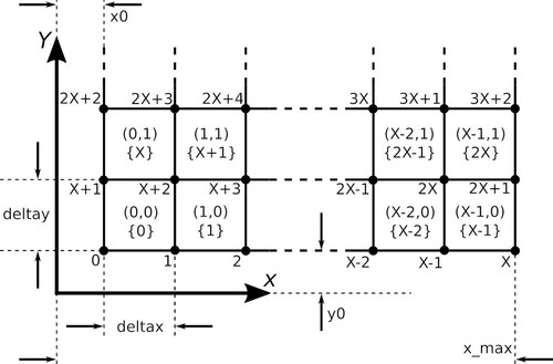

Figure 1. A diagram of the input parameters and the dimensions of the output surface to which they correspond.

Here parameters are hard-coded at the top of our Python script. Reading input from the terminal, a configuration file, or GUI could provide a better user experience but are not discussed here.

The parameters X and Y specify the number of cells to use in their respective directions. With these details we can calculate the x and y dimensions of each cell. We calculate cell widths below.

deltax = (x_max - x0) / float(X)
deltay = (y_max - y0) / float(Y)

The use of float() is not strictly necessary, but ensures that division takes place between floating point values rather than integers which on Python 2 discards remainders.

Just as for previous examples, we create instances of vtkPoints and vtkCellArray in which we store cells and points to define our surface.

points = vtk.vtkPoints()
cells = vtk.vtkCellArray()

We need to calculate all the points in the mesh. The surface is defined by quad cells and the pitch in the x and y directions is defined by deltax and deltay. We calculate each point on the surface using the formula provided in the programme input, then use these to define the mesh nodes. Each direction, x and y, has one node more than the number of cells in the corresponding direction. We therefore loop over X+1 and Y+1 points in each dimension.

zvals = []
for j in range(Y+1):
    for i in range(X+1):
        x = x0 + deltax*i
        y = y0 + deltay*j

        z_val = func_to_calculate(x, y)
        zvals.append(z_val)
        coord = x, y, z_val
        points.InsertNextPoint(coord)

The Z values above are stored in a list, zvals, for later use. We add points to the mesh using .InsertNextPoint(coord) on the vtkPoints collection. When this method is called VTK will automatically assign a global ID to the node. This ID can also be used to index the zvals list. This fact is used later when assigning scalar point data to mesh nodes.

for j in range(Y):
    for i in range(X):
        quad = vtk.vtkQuad()
        corner_id = get_id(i, j)

        quad.GetPointIds().SetId(0, corner_id)
        quad.GetPointIds().SetId(1, corner_id + 1)
        quad.GetPointIds().SetId(2, corner_id + (X+2))
        quad.GetPointIds().SetId(3, corner_id + (X+1))
        cells.InsertNextCell(quad)

A diagram of the global point IDs showing the numbering scheme for points.

Figure 2. The global point IDs of an arbitrary cell. The point on the lowest corner has an ID of N and the count of cells across the x-axis is used to calculate node IDs.

The next step is to create the vtkQuad cells in the polygon mesh. These cells have four local points with ID 0, 1, 2, and 3 which need to be associated with 4 global point IDs. Point IDs are assigned by VTK in the order in which they are inserted using points.InsertNextPoint(coord). Each node ID above is given by starting with N using i + j(X+1). The remaining node IDs are obtained using the values shown in the example mesh cell.

mesh = vtk.vtkPolyData()
mesh.SetPoints(points)
mesh.SetPolys(cells)

The point data is placed in a vtkDoubleArray. It is then set as the point data in the mesh.

point_data = vtk.vtkDoubleArray()
point_data.SetNumberOfComponents(1)

for zval in zvals:
    point_data.InsertNextTuple([zval])

mesh.GetPointData().SetScalars(point_data)

There are 2 new artefacts to the visualisation that we have not yet discussed. These are a box around the boundary of the mesh and coordinate axes. These help the user visualise and understand the plot. Both of these require that a vtkPolyDataNormals instance be derived from the polygon mesh. This information is easily generated using the mesh data:

norms_generator = vtk.vtkPolyDataNormals()
norms_generator.SetInputData(mesh)

Coordinate axes are then generated from this data.

axes = vtk.vtkCubeAxesActor2D()
axes.SetInputConnection(norms_generator.GetOutputPort())
axes.SetCamera(renderer.GetActiveCamera())
axes.SetLabelFormat("%1.1g")

Similarly the outline filter is created with the following.

outline_filter = vtk.vtkOutlineFilter()
outline_filter.SetInputConnection(norms_generator.GetOutputPort())

The axes are an Actor2D and can be added to the renderer just as for any other actor. The outline filter is a subclass of vtkPolyData, so it is connected to a vtkPolyDataMapper, a vtkActor, then added to the renderer with renderer.AddActor(outline_actor).

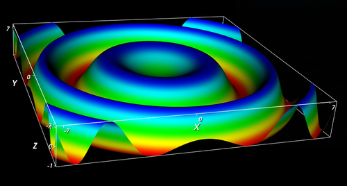
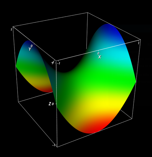
The final results are shown below.

Image of plot of function z = 0.2 * (x^2^ + y^2^).

Figure 3. Final result of the visualisation showing a plot of the function: f(x, y) = sin[0.2×(x² + y²)].

Image of plot of function z = x^2^ - y^2^.

Figure 4. Plot of function f(x, y) = x² - y². The only change is the function provided as input data.

Continue here for a description of colour models and how they are used in VTK.

VTK: Example plotting application

An application created with VTK. We build on the previous topics covered in this series.